Soaring technology stocks led the longest bull market in history during the 1990s, driving investors to shun stocks of dividend-paying firms.
The steady stock performance of more conservative firms just seemed pale in comparison. But now, rising interest rates and slowing corporate earnings are causing investors to again turn to the tried-and-true: high-quality firms with strong cash flows, solid earnings and a healthy dividend stream.
Companies that can commit to paying a regular dividend are ones that generally are fundamentally strong and optimistic about their future. A company’s dividend history is a good indication of its willingness to share profits and demonstrate accountability to investors. In periods of market uncertainty, these qualities become especially appealing to investors.
Stocks of companies that pay dividends generally have less price fluctuation than stocks of non-dividend payers. The dividend can create a cushion and smooth out a stock’s price volatility. It’s important to remember, however, that although dividend-paying stocks can add diversification to your portfolio and help minimize volatility, they still involve risk.
The 2003 Tax Act added allure to dividend-paying stocks. It lowered the tax rate for individuals on qualified dividends from as much as 38.6 percent to just 15 percent, depending on your income tax bracket.
This appreciation for dividends has spawned a renewed interest in mutual funds that pay dividends like the American Century Equity Income Fund (TWEIX), which has been investing in dividend-paying stocks for more than a decade. The companies in the fund typically are well-established and fundamentally strong, have steady earnings, a solid balance sheet and a history of paying dividends.
The size of dividends also is on the rise. Three quarters of the companies in the S&P 500 Index pay dividends, and more than half of them increased their payouts during 2004. That’s proof of a lot of strong balance sheets. A business has to have the earnings to pay a dividend and a strong balance sheet to increase one.
Investors’ preference for dividend-paying stocks is likely to continue, and so will the ability of many companies to continue paying dividends. Several years of economic uncertainty have driven companies to cut costs, reduce debt and rein in their capital spending. That means many of them now have a lot of cash on their balance sheets.
This combination of lower debt and larger cash pools gives them the ability to increase dividends. Even with the current emphasis returning more cash to shareholders, the current dividend payout ratio is still below the historical average.
Wednesday, January 27, 2016
Tuesday, March 31, 2015
The Head and Shoulders Pattern Forms
The Head and Shoulders pattern forms after an uptrend, and if confirmed, marks a trend reversal. The opposite pattern, the Inverse Head and Shoulders, therefore forms after a downtrend and marks the end of the downward price movement. In the current article we will only discuss the Head and Shoulders pattern, because the inverse variety is its twin, but from a bullish point of view.
As you can guess by its name, the Head and Shoulders pattern consists of three peaks – a left shoulder, a head and a right shoulder. The head should be the highest (what an abomination it would be otherwise) and the two shoulders should be at least relatively of equal height. As the price corrects from each peak, the lows it retreats to form the so-called neckline, which is later used for confirming the pattern (we will get to that soon enough). Here is how an H&S pattern looks like.

As you can guess by its name, the Head and Shoulders pattern consists of three peaks – a left shoulder, a head and a right shoulder. The head should be the highest (what an abomination it would be otherwise) and the two shoulders should be at least relatively of equal height. As the price corrects from each peak, the lows it retreats to form the so-called neckline, which is later used for confirming the pattern (we will get to that soon enough). Here is how an H&S pattern looks like.
Wednesday, November 12, 2014
Simple Moving Average
In technical analysis the most commonly used type of moving average is the simple moving average (SMA), which is sometimes called an arithmetic moving average. It is referred to as ”simple”, because it uses a simple way of averaging. A SMA is usually constructed by adding a set of data and then dividing it by the number of observations during the period, which is being examined.
How to estimate the value of a simple moving average?
In order to estimate the value of a simple moving average, we need the following:
First, to define a number of trading sessions (periods), which will be used in the calculation. Let us use the 10 most recent trading days (sessions).
Second, to decide what type of prices we shall use. Most moving averages of prices are based on closing prices, but these averages could also be estimated with the use of highs, lows, daily means etc. Let us use the closing prices in our case.
Third, to calculate a simple average value of these prices.
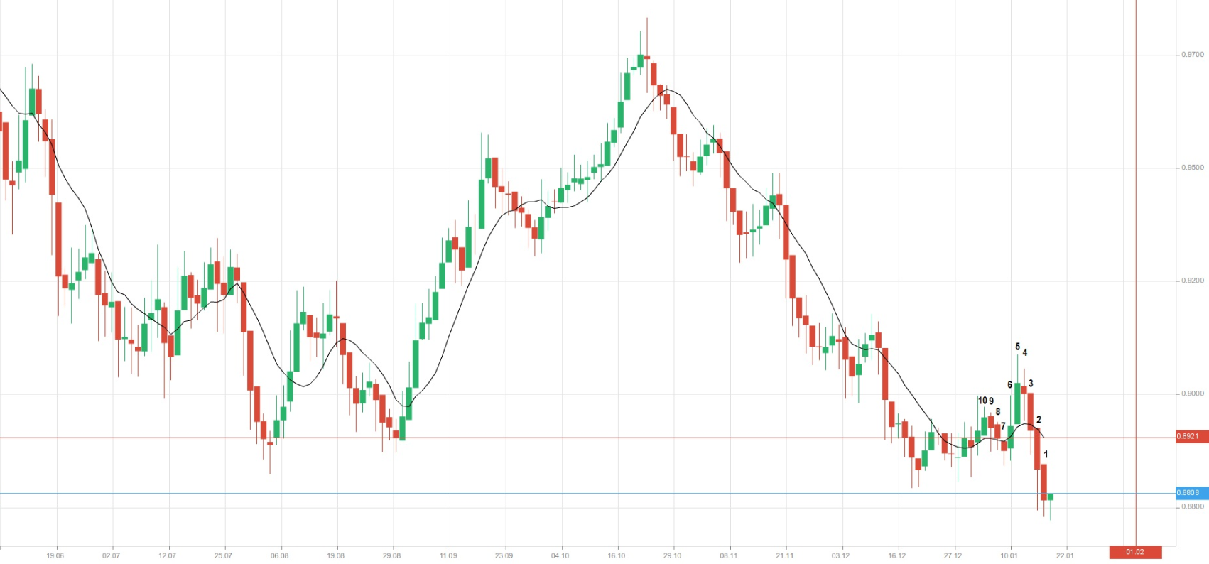
Let us look at the following graph (graph 1).
 On the chart above we can see a 10-day simple moving average (the black line), with its value shown in the red rectangle (0.8921). The marked candles represent the periods (10 days, because we use a daily chart), which closing prices take part in the calculation of the SMA. We count the candles in the opposite direction, because moving averages take into account the most recent number of periods. The most recent green candle has no SMA, because the trading day is not over yet and, respectively, there is no closing price. Therefore, it cannot be used in our calculation. Tomorrow, in order to estimate the SMA value, candle 10 will be replaced with the current-day candle, which will already be closed. It is how the moving average indicator moves across the graph.
Now, let us present the close prices of the 10 marked candles. We have to sum all the close prices and divide the sum by the number of periods (days).
So, the 10-day SMA has a value of 0.8921, exactly the same as shown in the rectangle above.
What do we mean when saying that the SMA is moving across price action?
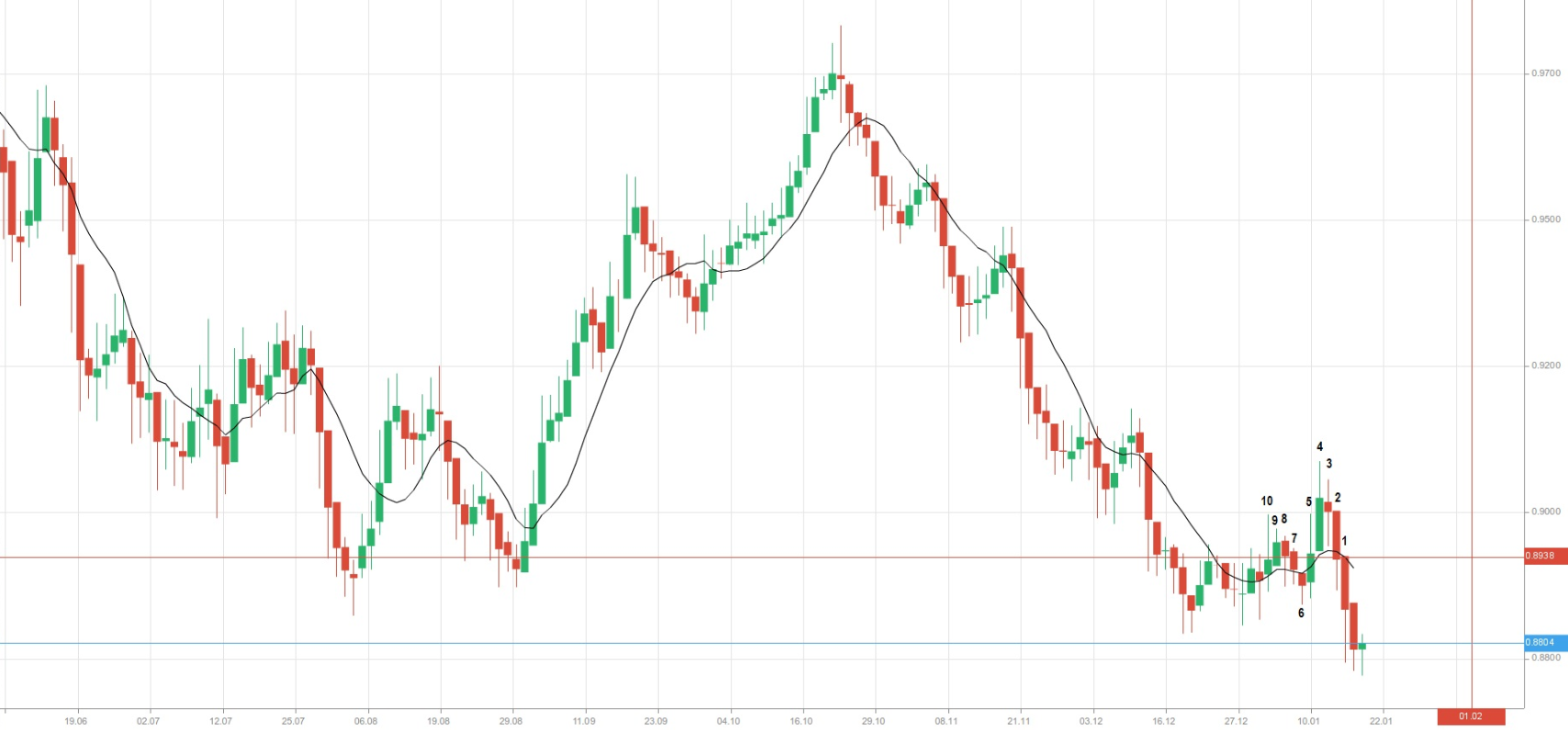
Let us move one day back and imagine the same situation as above. Now candle number 1 on graph 1 will not be taken into consideration when calculating the new SMA, as it has not yet closed. At the same time, we should take into account the candle, which stands before candle number 10 on graph 1.

So, the new 10-day SMA has a value of 0.8938. What can we observe in the table above? It seems that all the close prices remain the same with the exception of just one – that of the 10th day. Tomorrow, when calculating the SMA, the trading platform will replace candle number 10 on graph 1 with the most recent candle, or the candle for the current day.
Beginner traders should note that simple moving averages can be calculated for different time frames. In case we use a 15-min chart, where each candle stands for a 15-minute period, the SMA indicator will show the average closing price for the past 10 periods, or 150 minutes. If we apply the SMA on a 1-hour chart, it will show the average closing price for the past 10 hours. This, of course, will be valid, if we keep the period number unchanged.
How to estimate the value of a simple moving average?
In order to estimate the value of a simple moving average, we need the following:
First, to define a number of trading sessions (periods), which will be used in the calculation. Let us use the 10 most recent trading days (sessions).
Second, to decide what type of prices we shall use. Most moving averages of prices are based on closing prices, but these averages could also be estimated with the use of highs, lows, daily means etc. Let us use the closing prices in our case.
Third, to calculate a simple average value of these prices.
Let us look at the following graph (graph 1).
Now, let us present the close prices of the 10 marked candles. We have to sum all the close prices and divide the sum by the number of periods (days).
| Trading Day | Close Price |
| 1 | 0.87777 |
| 2 | 0.88196 |
| 3 | 0.89143 |
| 4 | 0.89649 |
| 5 | 0.90522 |
| 6 | 0.89942 |
| 7 | 0.88975 |
| 8 | 0.88993 |
| 9 | 0.89257 |
| 10 | 0.89665 |
| 10-day SMA | 0.89212 |
So, the 10-day SMA has a value of 0.8921, exactly the same as shown in the rectangle above.
What do we mean when saying that the SMA is moving across price action?
Let us move one day back and imagine the same situation as above. Now candle number 1 on graph 1 will not be taken into consideration when calculating the new SMA, as it has not yet closed. At the same time, we should take into account the candle, which stands before candle number 10 on graph 1.
| Trading Day | Close Price |
| 1 | 0.88196 |
| 2 | 0.89143 |
| 3 | 0.89649 |
| 4 | 0.90522 |
| 5 | 0.89942 |
| 6 | 0.88975 |
| 7 | 0.88993 |
| 8 | 0.89257 |
| 9 | 0.89665 |
| 10 | 0.89450 |
| 10-day SMA | 0.89379 |
So, the new 10-day SMA has a value of 0.8938. What can we observe in the table above? It seems that all the close prices remain the same with the exception of just one – that of the 10th day. Tomorrow, when calculating the SMA, the trading platform will replace candle number 10 on graph 1 with the most recent candle, or the candle for the current day.
Beginner traders should note that simple moving averages can be calculated for different time frames. In case we use a 15-min chart, where each candle stands for a 15-minute period, the SMA indicator will show the average closing price for the past 10 periods, or 150 minutes. If we apply the SMA on a 1-hour chart, it will show the average closing price for the past 10 hours. This, of course, will be valid, if we keep the period number unchanged.
Simple moving averages may differ in length
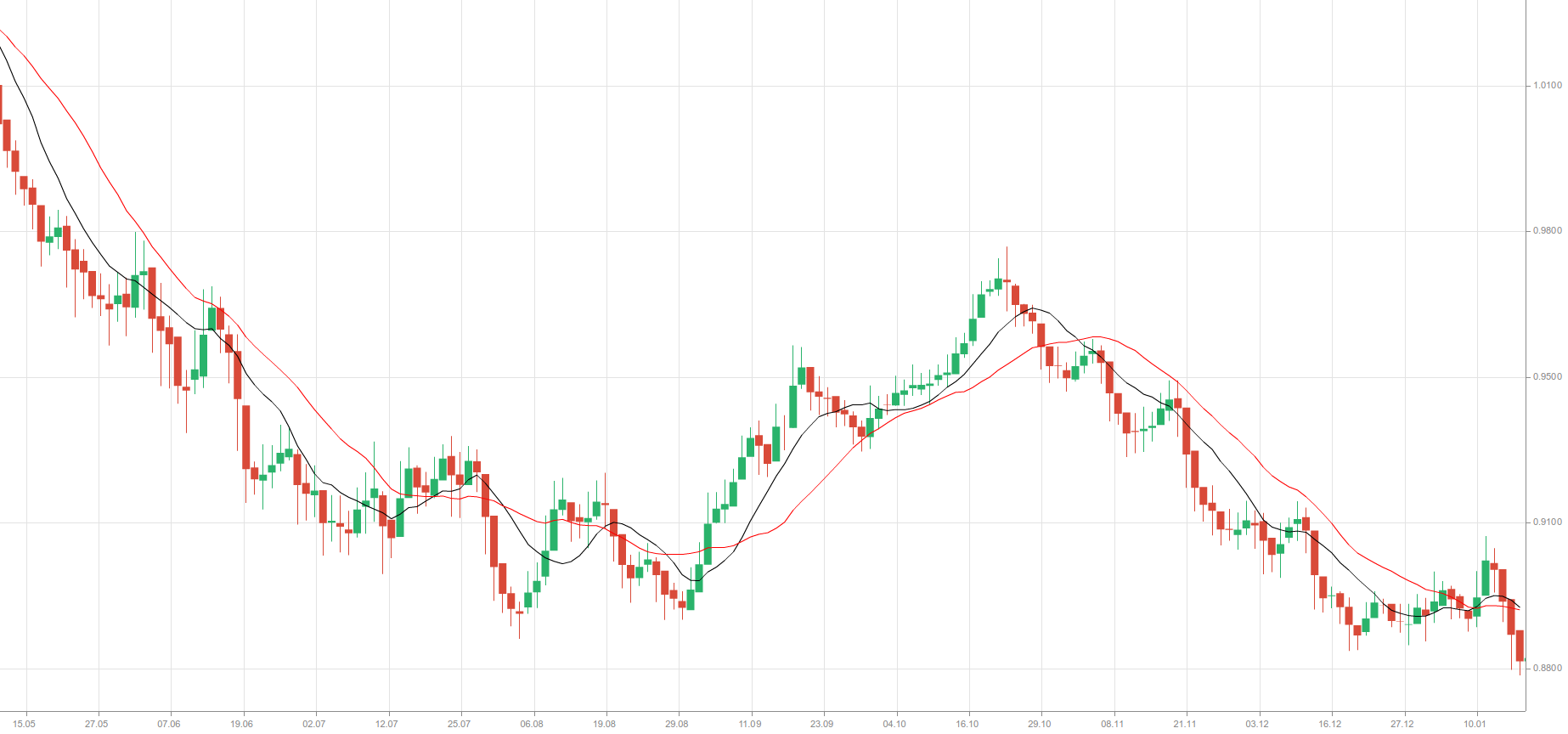
We can construct moving averages of different lengths. On the next graph we can see another moving average, a 20-day SMA (the red line). It is calculated by adding the 20 most recent closing prices and dividing the sum by 20.

Some of the most popular daily moving averages are for the periods of 200, 80, 50, 30, 20 and 10 days. These periods are considered as arbitrary and were chosen in the days before the invention of computers, when calculations had to be done by hand.
The 10-day, 20-day and 80-day moving averages represent approximately two weeks, one month and four months of trading data respectively.
Longer moving averages usually pick up changes in a trend more slowly, but yet, it is less likely that they will give a false signal for a trend change, because they represent a greater number of data observations, or more information. The more data we include in the calculation of the SMA, the less important each day’s data becomes in this calculation. A large change in the value of data during one day would not cause a large impact upon the longer-term moving average.
If we look again at the graph above, we can notice that the 10-day SMA demonstrates more variability than the longer, 20-day SMA. The latter is said to be the slower, the lazier moving average. It provides more smoothing, but it is also slower at indicating trend reversals.
We can construct moving averages of different lengths. On the next graph we can see another moving average, a 20-day SMA (the red line). It is calculated by adding the 20 most recent closing prices and dividing the sum by 20.
Some of the most popular daily moving averages are for the periods of 200, 80, 50, 30, 20 and 10 days. These periods are considered as arbitrary and were chosen in the days before the invention of computers, when calculations had to be done by hand.
The 10-day, 20-day and 80-day moving averages represent approximately two weeks, one month and four months of trading data respectively.
Longer moving averages usually pick up changes in a trend more slowly, but yet, it is less likely that they will give a false signal for a trend change, because they represent a greater number of data observations, or more information. The more data we include in the calculation of the SMA, the less important each day’s data becomes in this calculation. A large change in the value of data during one day would not cause a large impact upon the longer-term moving average.
If we look again at the graph above, we can notice that the 10-day SMA demonstrates more variability than the longer, 20-day SMA. The latter is said to be the slower, the lazier moving average. It provides more smoothing, but it is also slower at indicating trend reversals.
SMA and the trend
Moving averages are valuable, as they smooth daily fluctuations, allowing the technical analyst to see the underlying trend without being distracted by the small (daily) movements. A rising moving average usually signals an uptrend, while a falling moving average indicates a downtrend. Some analysts have adopted the following approach, when it comes to relating the SMA with a particular trend: If the close price of a tradable instrument is above some simple moving average, then the trend must be bullish. If the close price is below some simple moving average, then the trend must be bearish. However, choosing a period for trend estimation is a matter of personal preferences. The period of the SMA will depend on one’s trading style and time frame for trading. Thus, choosing the appropriate period comes with experimentation and, of course, experience.
Despite that simple moving averages provide help when identifying a trend, they do so after the trend has begun. Therefore, moving averages are lagging indicators, as they are based on past prices.
Subscribe to:
Posts (Atom)